Environmental Measurements and Quantum Trajectories in Metastable Open Systems

Summer 2026 Research Internship | Jack Group, University of Cambridge

Overview

This project investigated how environmental measurement schemes affect the quantum trajectories of a driven, metastable two-qubit open quantum system. Although a Lindblad master equation specifies the evolution of the unconditional density matrix, monitoring the environment yields individual, stochastic, conditioned trajectories. Distinct measurement prescriptions can produce very different trajectories even when they give the same unconditional dynamics.

I explored quantum-jump and diffusive unravellings, changes to the measurement parameter, the distinction between separate and combined decay channels, and the spectral properties governing evolution between jumps.

My contribution

I independently implemented and ran the numerical simulations, generated the figures, and analysed the results. I met with my supervisor weekly to discuss findings, assess interpretations, and identify the next questions to investigate.

Tools: Python, QuTiP, NumPy, SciPy and Matplotlib.

Physical model

Assuming Markovian Lindblad dynamics and using units where $\hbar=1$, the unconditional density matrix evolves according to

$$\frac{d\rho}{dt}=-i[H,\rho]+\sum_k\left(J_k\rho J_k^\dagger-\frac{1}{2}\{J_k^\dagger J_k,\rho\}\right).$$

The driven two-qubit model has Hamiltonian

$$H=\Omega_1\sigma_1^y+\Omega_2\sigma_2^y,\qquad \Omega_i=\varepsilon\omega_i,$$

with two decay channels,

$$J_1=\sqrt{\gamma_1}\,n_1\sigma_2^-,\qquad J_2=\sqrt{\gamma_2}\,(1-n_1)\sigma_2^+.$$

Here $n_1$ projects onto the excited state of the first qubit. Each detected quantum jump resets the system to one of two basis states: $J_1$ maps the system to $\lvert 10\rangle$, while $J_2$ maps it to $\lvert 01\rangle$.

The two jump operators share a two-dimensional dark subspace, spanned by $\lvert 01\rangle$ and $\lvert 10\rangle$, which they both annihilate:

$$\mathcal{H}_{\mathrm{DFS}} = \operatorname{span}\{\lvert 01\rangle,\lvert 10\rangle\}.$$

In the absence of driving ($\epsilon=0$), this constitutes an exact decoherence-free subspace (DFS). For weak but finite driving, the Hamiltonian couples these dark states to the dissipative states $\lvert 00\rangle$ and $\lvert 11\rangle$, allowing occasional quantum jumps. This weak coupling between the dark and dissipative sectors gives rise to long-lived metastable behaviour.

The metastable behaviour can also be understood through the spectrum of the Liouvillian $\mathcal{L}$, defined by $\dot{\rho}=\mathcal{L}(\rho)$. In the absence of driving, the DFS gives rise to four stationary eigenoperators of $\mathcal{L}$. Weak driving lifts this degeneracy, leaving one zero eigenvalue corresponding to the stationary state and three slowly decaying modes, separated from the remaining fast modes by a spectral gap.

Consequently, the system initially relaxes rapidly towards a metastable manifold, spanned by the four slow eigenoperators. It then evolves within this manifold on a much longer timescale, before eventually reaching its unique stationary state.

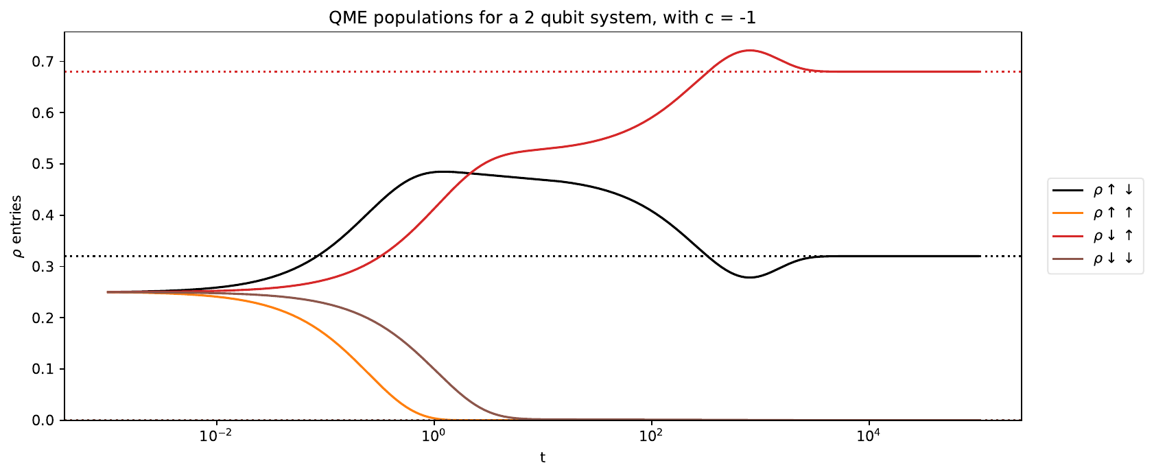
The corresponding unconditional master-equation solution is shown below. Unlike individual quantum trajectories, the master-equation dynamics are independent of the measurement parameter $c$, provided the Hamiltonian is transformed accordingly.

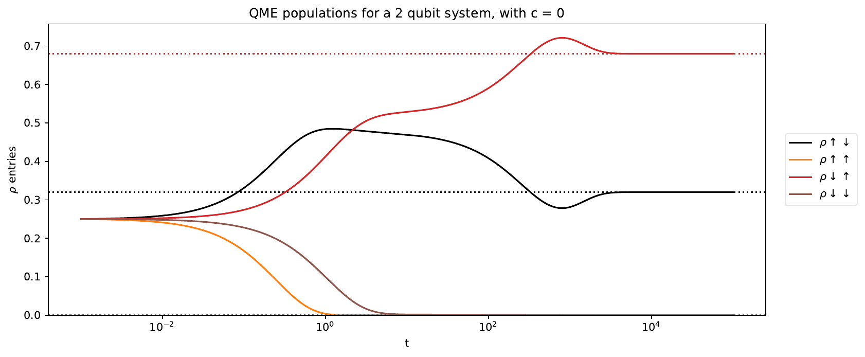
View an example master-equation solution for c = -1

Stochastic Schrödinger equation and MCWF method

To investigate individual conditioned trajectories, I used the Monte Carlo wave-function (MCWF) approach, which numerically unravels the master equation into realisations of a stochastic Schrödinger equation (SSE).

For the quantum-jump unravelling, the system evolves under a non-Hermitian effective Hamiltonian between randomly occurring detection events. The probability of a jump through channel $k$ during an interval $dt$ is

$$dp_k = \langle\psi|J_k^\dagger J_k|\psi\rangle\,dt.$$

Following a detected jump, the wavefunction is updated according to

$$|\psi\rangle \longrightarrow \frac{J_k|\psi\rangle} {\sqrt{\langle\psi|J_k^\dagger J_k|\psi\rangle}}.$$

Averaging over many independently sampled trajectories recovers the unconditional density matrix,

$$\rho(t)=\mathbb{E}\left[|\psi(t)\rangle\langle\psi(t)|\right].$$

This provides a way to examine individual measurement-conditioned histories while retaining consistency with the Lindblad master equation.

Numerical investigations and results

1. Changing the environmental measurement scheme

For a single jump channel, consider the transformation

$$J_c=J+cI,\qquad H_c=H+\frac{ic}{2}(J^\dagger-J),\qquad c\in\mathbb{R}.$$

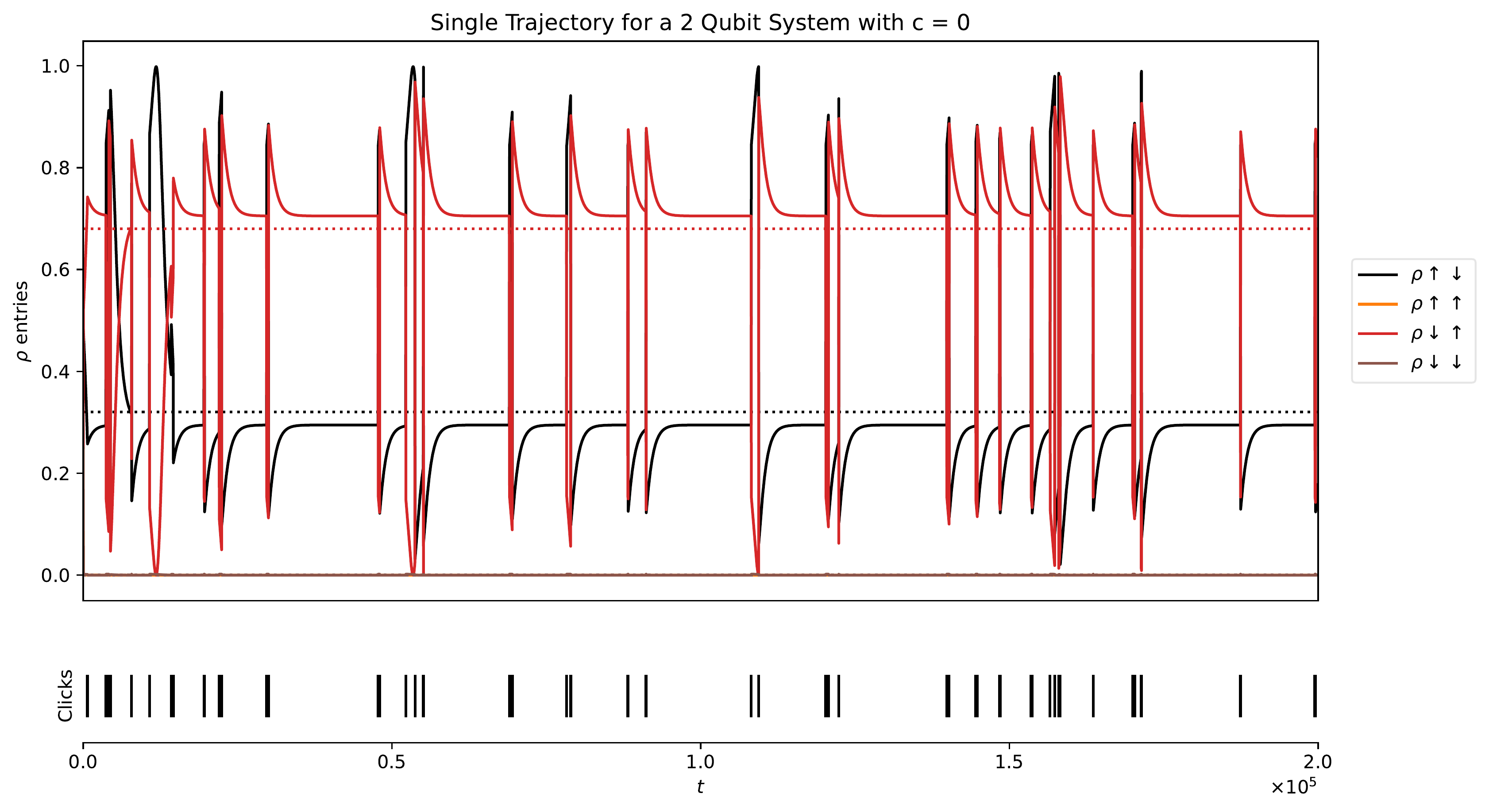
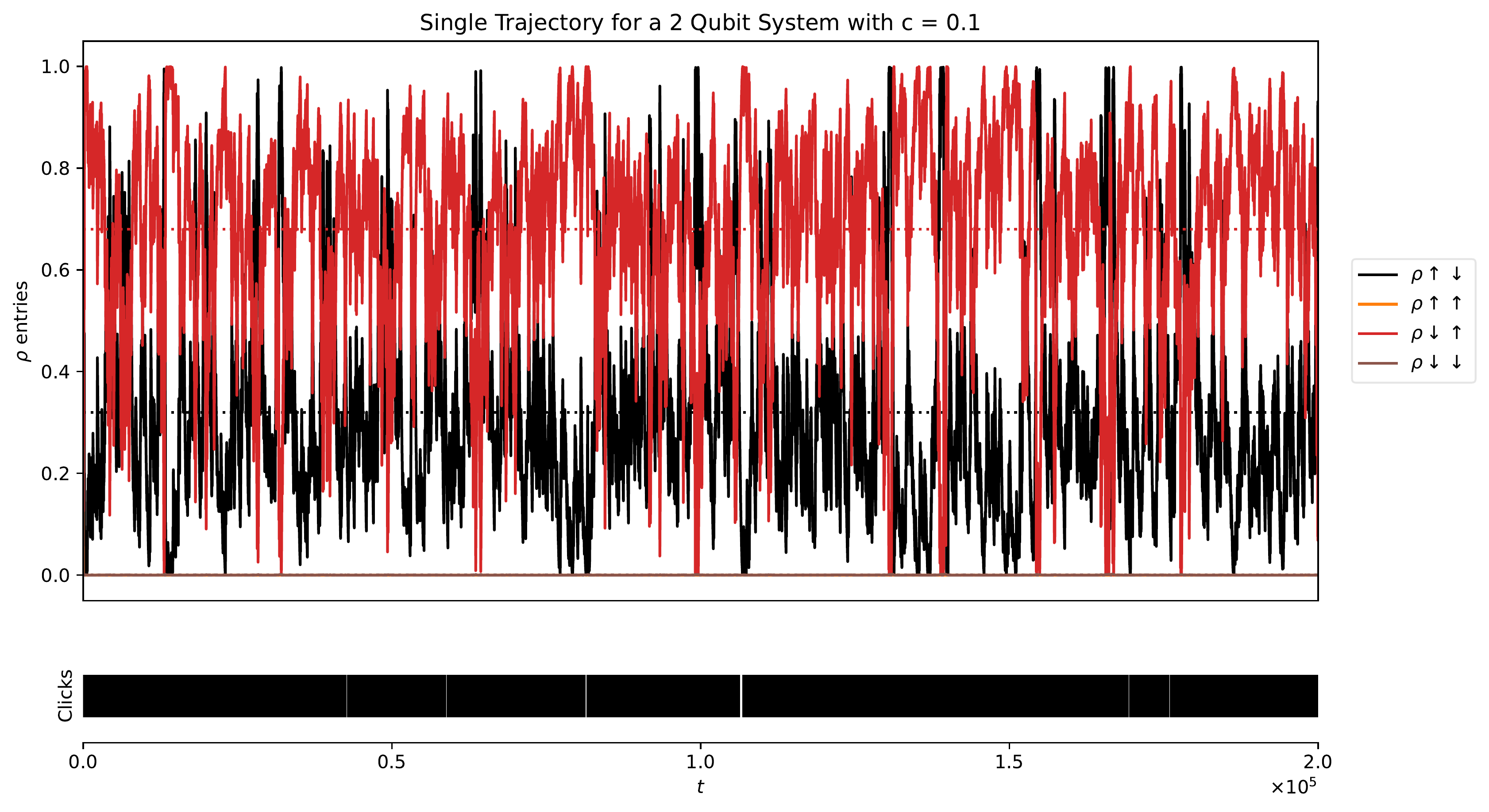
This transformation leaves the Lindblad master equation unchanged, but significantly alters the conditioned quantum trajectories. Increasing the measurement parameter $c$ increases the frequency of quantum jumps while reducing the change in the state associated with each jump. In the large-$c$ limit, the jump rate scales as $c^2$, while the state change per jump scales as $1/c$. The system therefore undergoes increasingly frequent but smaller jumps, approaching diffusive behaviour.

This is illustrated by comparing individual trajectories at $c=0$ and $c=0.1$. Despite their very different appearances, both unravel the same unconditional master equation, as the transformation of the jump operator is accompanied by a compensating change in the Hamiltonian.

Individual trajectories for $c=0$ and $c=0.1$:

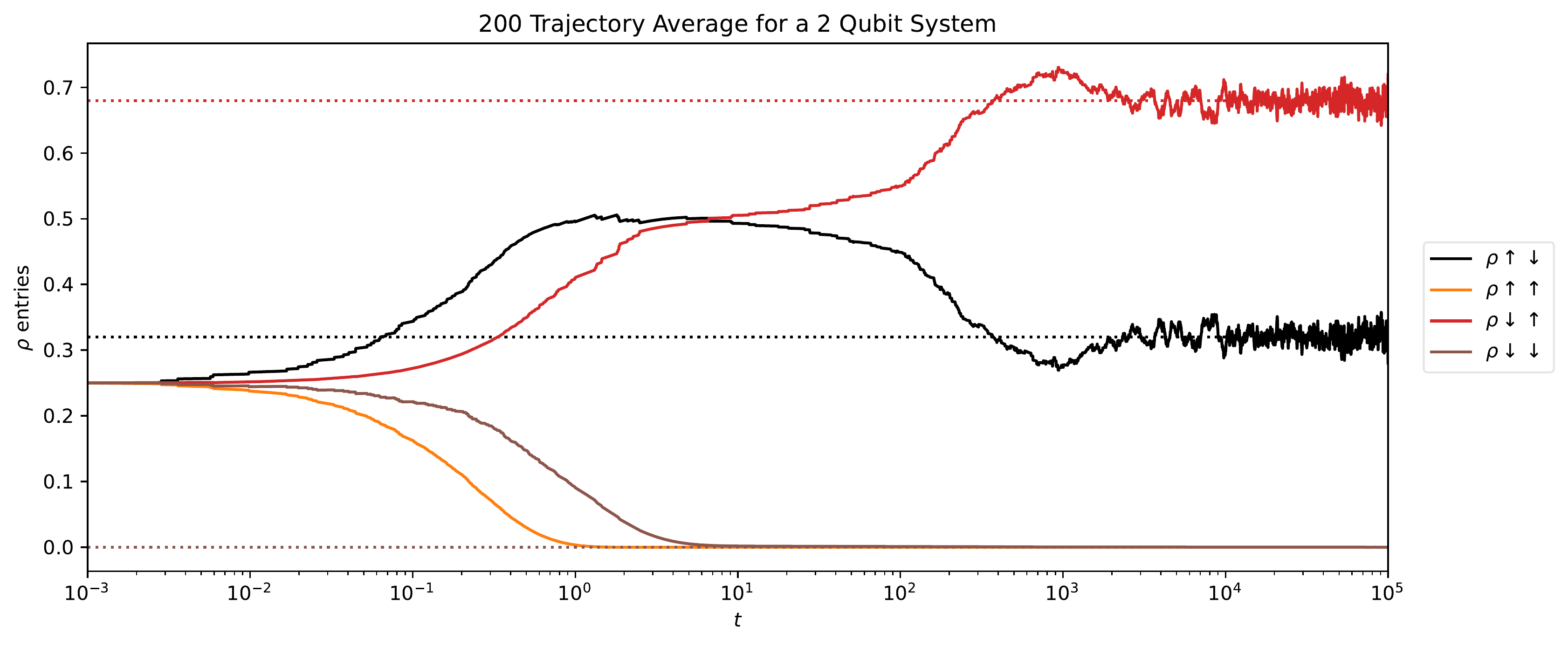
Averaging over independent stochastic trajectories approaches the unconditional master-equation solution. The following example averages 200 trajectories; residual differences reflect finite sampling.

2. Homodyne and heterodyne detection

I also investigated diffusive unravellings. In contrast to direct photon counting, homodyne detection continuously measures a field quadrature, producing noisy but continuous conditioned evolution. Heterodyne detection monitors two quadratures, introducing two independent noise components.

For ideal homodyne detection, the conditioned state evolves according to the stochastic Schrödinger equation

$$\begin{aligned} d|\psi\rangle ={}& \left[ -iH-\frac{1}{2}\sum_k \left( J_k^\dagger J_k -2\langle X_k\rangle J_k +\langle X_k\rangle^2 \right) \right]|\psi\rangle\,dt\\ &+\sum_k \left(J_k-\langle X_k\rangle\right) |\psi\rangle\,dW_k, \end{aligned}$$

where $X_k=(J_k+J_k^\dagger)/2$ is the measured field quadrature and $dW_k$ are independent real Wiener increments representing measurement noise. This assumes ideal detection with zero local-oscillator phase.

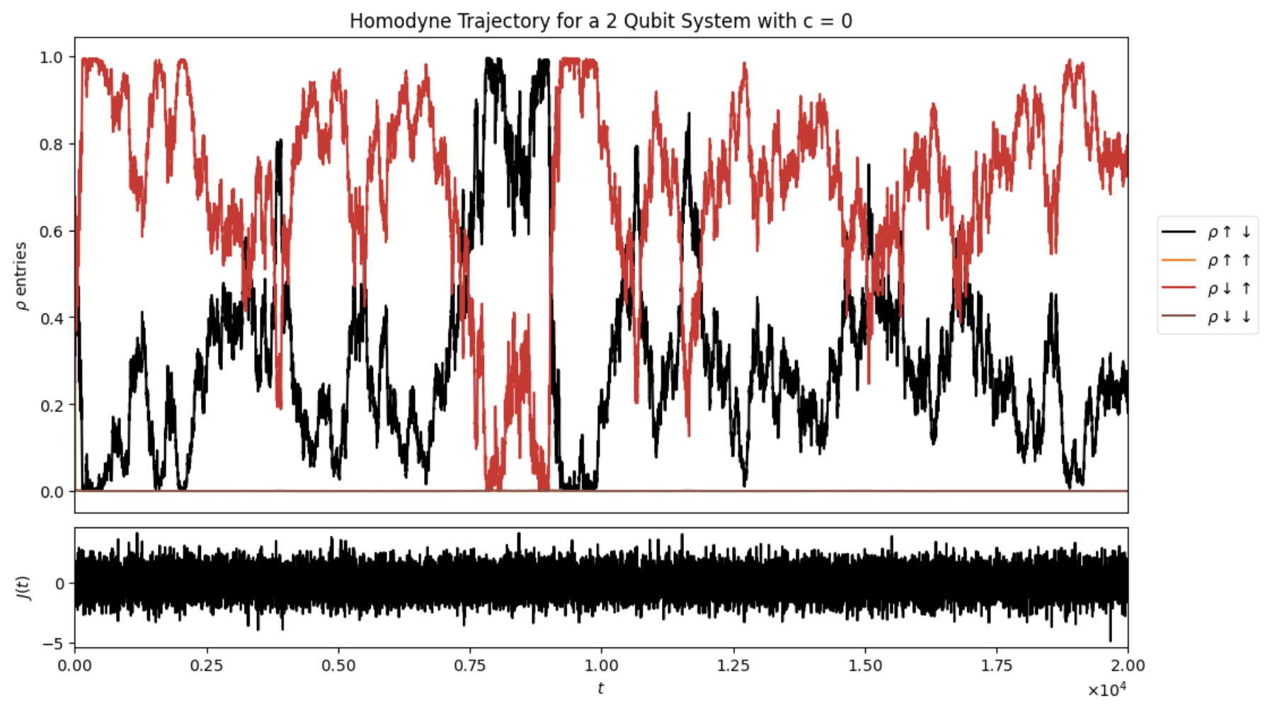
Importantly, the quantum-jump unravelling approaches homodyne detection in the large-$c$ limit. As $c$ increases, the jump rate scales as $c^2$, while the change in the state associated with each jump scales as $1/c$. Consequently, jumps become increasingly frequent but progressively smaller. In the limit $c\to\infty$, the transformed jump channel converges to continuous diffusive evolution, with any untransformed channels retaining their jump dynamics.

I compared homodyne trajectories with jump-based trajectories at larger values of $c$, demonstrating how the discrete jump process approaches diffusive behaviour.

3. Separate versus combined jump operators

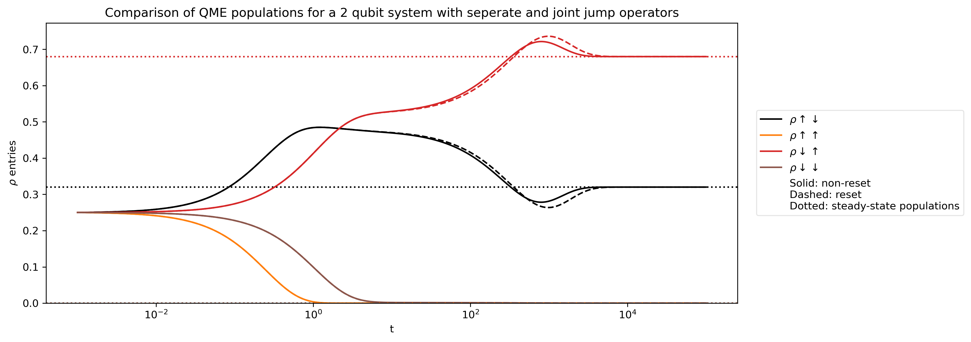
I compared monitoring two channels with operators $J_1$ and $J_2$ against using one combined operator $J=J_1+J_2$. With separate channels, jumps reset the state to specific basis states; with the combined channel, the post-jump state may be a superposition.

Importantly, combining the two operators is not the same as the gauge transformation above. The dissipator of $J_1+J_2$ includes cross terms, so the unconditional dynamics can change. My simulations showed differences in transient coherences and populations, while the two models approached the same steady state for the parameters studied.

4. No-jump dynamics and generator spectra

Between detection events, the unnormalised state follows non-unitary evolution generated by an effective Hamiltonian:

$$H_{\mathrm{eff}}=H_c-\frac{i}{2}\sum_k J_{k,c}^\dagger J_{k,c},\qquad G=-iH_{\mathrm{eff}},\qquad \lvert\widetilde{\psi}(t)\rangle=e^{Gt}\lvert\psi(0)\rangle.$$

Since the dynamics preserve real amplitudes, the normalised two-qubit state can be represented as a point on the three-sphere $S^3$, embedded in four-dimensional real space. Equivalently, three amplitudes specify a point inside a three-dimensional unit ball, with the fourth determined up to a sign by normalisation. Between jumps, the state evolves deterministically along a continuous path on this sphere, while detection events cause discontinuous jumps to new points.

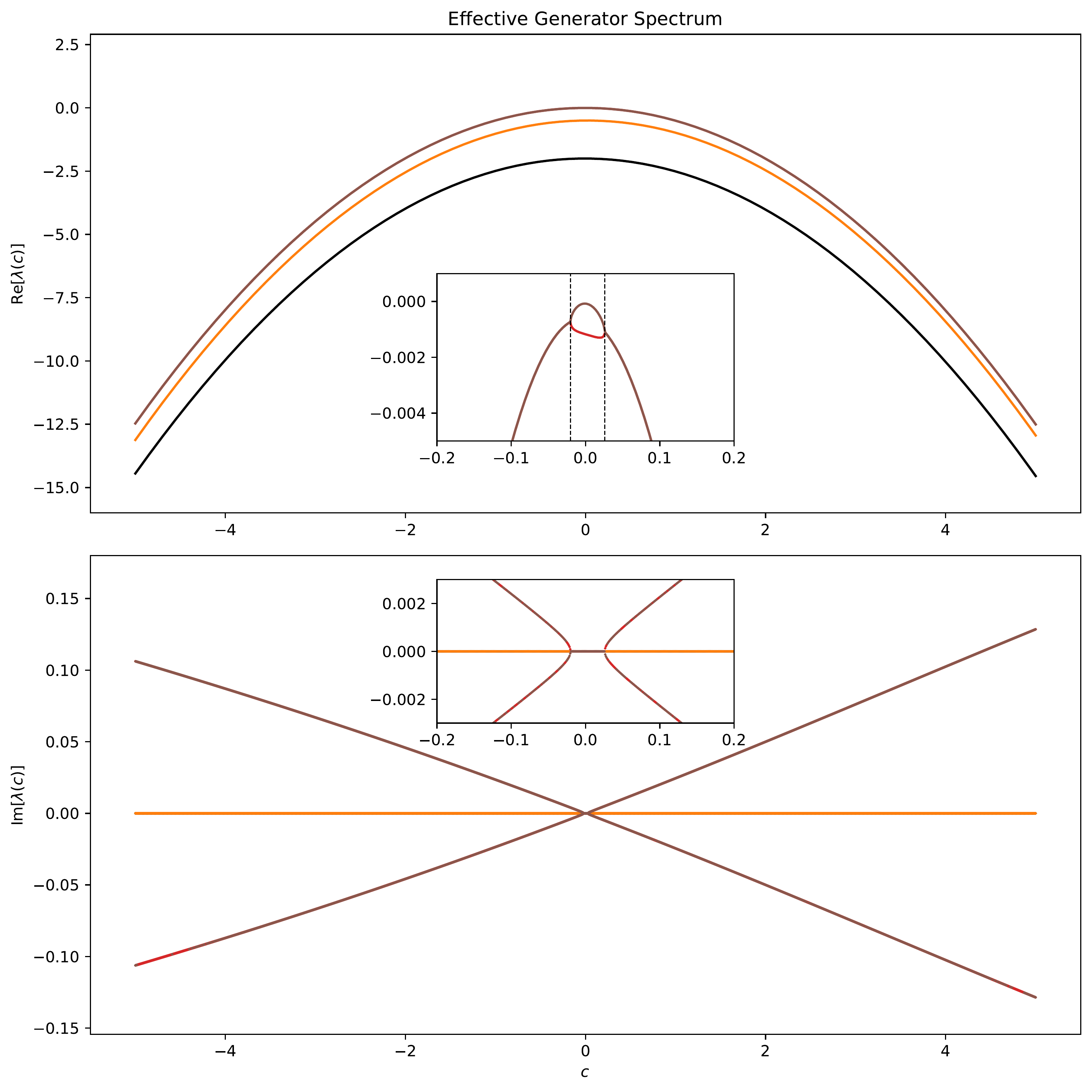
I studied the spectrum of $G$ as the measurement parameter varied. Eigenvalues with the largest real parts govern the dominant long-time contributions to the no-jump evolution. When leading eigenvalues share the same real part, different imaginary parts can produce oscillatory rather than stationary asymptotic behaviour, provided the corresponding modes are populated.

View an example no-jump path at c = 0.1

Takeaway

The project highlighted the distinction between a system’s unconditional density-matrix dynamics and the individual histories inferred from monitoring its environment. Measurement transformations may leave the Lindblad equation invariant while substantially changing trajectories, whereas combining physically distinct jump channels can modify the master equation itself. The spectrum of the effective non-Hermitian generator provides insight into the evolution between detected jumps.

Acknowledgements

I would like to thank Professor Rob Jack for his supervision and guidance throughout this research, and the Ian McDonald Fund at Trinity College, Cambridge, for its generous financial support.

This page presents selected figures and a summary of my computational research. The simulation source code is not included.